Conjuring Nature’s Chaos on a Deterministic Machine: Perlin Noise

15/03/2026 · tags: c, low-level, determinism, and physics

noiz Logo

In a philosophical sense, determinism is the belief that every event is the inevitable consequence of prior causes — governed by a fixed set of rules. In a deterministic system, the current state, combined with a defined set of inputs, fully determines every future state. Given enough information, the entire trajectory of such a system becomes knowable in advance.
This is precisely what makes computers so powerful. A CPU is a deterministic machine: same inputs, same internal state, same output — every single time. For most engineering problems, this predictability is a feature, not a limitation. You can reason about your program’s behavior, trace bugs, and anticipate what comes next. But this strength becomes a constraint when your goal is to mimic nature.

Consider cigarette smoke curling through still air, the jagged silhouette of a mountain range, or the surface texture of weathered bark. These phenomena appear unpredictable — not because nature is fundamentally lawless, but because the underlying systems are so high-dimensional and sensitive to initial conditions that they become practically intractable.

Classical physics is itself deterministic; this is the core of Laplace’s argument that a sufficiently informed intellect could predict the entire future of the universe. True non-determinism only enters the picture at the quantum level. So the problem isn’t that nature is random — it’s that nature is complex beyond practical simulation. This raises the central question: how do you produce apparently unpredictable outputs on a machine that is, by design, fully predictable?

Is rand() actually generates random numbers?

The short answer is no. rand() or similar random number methods from other libraries aren’t actually random. When we talk about randomness in computers, what we’re really talking about are pseudo-randoms. rand and similar methods work this way, using PRNG algorithms. Basically, these algorithms take a specific seed value and hash it until it’s unrecognizable. So, the process actually works by mimicking a certain randomness. But in the end, none of what’s created is truly random and predictable.

The problem here is that all this simulated randomness, in areas where you really expect there to be very few patterns—whether it’s an organic surface or a mountain—looks quite synthetic and doesn’t produce the desired result.

What Ken Perlin Fixed?

As you can see in the first image I added above, if you assign the value rand() % 255 to each pixel, you create white noise. The resulting image, resembling TV static, has very sharp lines, but the neighboring pixels have no relation to each other; it’s quite artificial and fundamentally predictable.

However, as mentioned above, objects in nature are not separated by such clear lines. Perlin actually solved this problem, managing to produce data that appears natural while still remaining pseudo-random and still operating within a deterministic machine.

How Actually The Algorithm Works?

To explain how the algorithm works, I started writing my own small PoC program, noiz. Here, we will try to partition the 2-dimensional space step by step, while remaining faithful to the original algorithm.

Basically, I started by adding 4 corner edges to a point P(x, y) that I chose in the plane.

noiz Logo

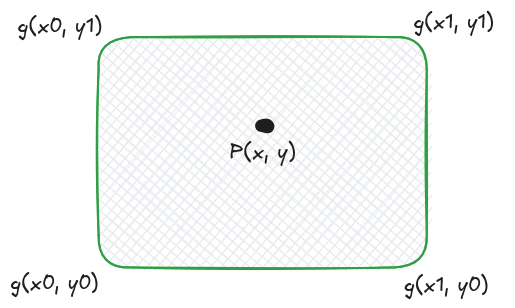
Here I divided the x and y points I have by the grid scale I determined. Let’s say we chose point P(50, 50) on a 100x100 plane with a grid size of 10. In this case, the corners of our point will be as follows:

UL grid:(5,5) pixel:(50,50)
UR grid:(6,5) pixel:(60,50)
LL grid:(5,6) pixel:(50,60)
LR grid:(6,6) pixel:(60,60)

The reason we chose four corners at our location is because these corners will later play a role in determining the noise at that point.

Gradient vectors to be more natural

As the next step, I continued by assigning a gradient vector to each of these corner points I selected. The purpose of using a gradient vector here, unlike the rand() function, is to create a connection between neighboring pixels. While there is no relationship between neighbors when only rand() is used, the gradient vector both establishes this relationship and assigns a flow direction to the connected pixels. This direction can be found in many things in nature; wind, water, or blood…

...
	vec2i_t g_upper_left = get_grid_corner(ix, iy, UPPER_LEFT, GRID_SIZE);
	vec2i_t g_upper_right = get_grid_corner(ix, iy, UPPER_RIGHT, GRID_SIZE);
	vec2i_t g_lower_left = get_grid_corner(ix, iy, LOWER_LEFT, GRID_SIZE);
	vec2i_t g_lower_right = get_grid_corner(ix, iy, LOWER_RIGHT, GRID_SIZE);

	vec2f_t g_upper_left_gradient =
		assign_gradient(g_upper_left.x, g_upper_left.y);
	vec2f_t g_upper_right_gradient =
		assign_gradient(g_upper_right.x, g_upper_right.y);
	vec2f_t g_lower_left_gradient =
		assign_gradient(g_lower_left.x, g_lower_left.y);
	vec2f_t g_lower_right_gradient =
		assign_gradient(g_lower_right.x, g_lower_right.y);
...

vec2f_t assign_gradient(int gx, int gy)
{
	int h = hash2d(gx, gy) & 7;

	return gradients[h];
}

For each point, I first convert the value I receive into a hash function to generate a pseudo-random number. Then, I assign this pseudo-random number as an index between a previously defined gradient vector and determine a random direction for each corner point. The resulting corner points look like this:

noiz Logo

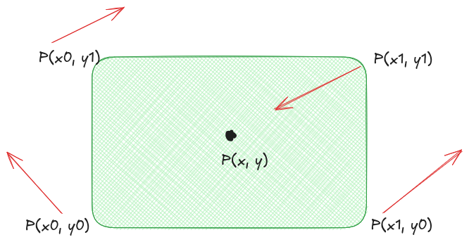
The gradient values for our point P(50, 50) are as follows:

UL grid:(5,5) pixel:(50,50) gradient:(-0.707000,0.707000)
UR grid:(6,5) pixel:(60,50) gradient:(0.707000,-0.707000)
LL grid:(5,6) pixel:(50,60) gradient:(0.707000,-0.707000)
LR grid:(6,6) pixel:(60,60) gradient:(0.000000,-1.000000)

Offset vectors to deceide which gradient has more impact

The offset vector answers the question: where is the pixel relative to the corner? The gradient vector tells you the direction of the corner. But you don’t know how effective that direction is for this pixel. Is the pixel close to the corner or far from it? In which direction?

The offset vector carries this information. Then, when you perform a dot product with the gradient, you get the answer to the question, “How well does the gradient direction of this corner match the position of this pixel?” So, without the offset, you wouldn’t have a second vector to perform a dot product with, only the gradient would remain — and this wouldn’t give you different values on a pixel-by-pixel basis; the entire grid square would have the same value.

...
	vec2f_t ul_offset = diff_from_corner(ul_pixel, x, y);
	vec2f_t ur_offset = diff_from_corner(ur_pixel, x, y);
	vec2f_t ll_offset = diff_from_corner(ll_pixel, x, y);
	vec2f_t lr_offset = diff_from_corner(lr_pixel, x, y);
...

vec2f_t diff_from_corner(vec2i_t corner_pixel, float x, float y)
{
	return (vec2f_t){ .x = (x - corner_pixel.x) / GRID_SIZE,
			  .y = (y - corner_pixel.y) / GRID_SIZE };
}

Using the simple method above, I first convert the selected corner points into 2D pixel values and then subtract them from our target point P(x,y).

Let’s look at the values again for our point P(50,50):

UL grid:(5,5) pixel:(50,50) gradient:(-0.707000,0.707000) offset:(0.000000,0.000000)
UR grid:(6,5) pixel:(60,50) gradient:(0.707000,-0.707000) offset:(-1.000000,0.000000)
LL grid:(5,6) pixel:(50,60) gradient:(0.707000,-0.707000) offset:(0.000000,-1.000000)
LR grid:(6,6) pixel:(60,60) gradient:(0.000000,-1.000000) offset:(-1.000000,-1.000000)

Now our point is at x=50 and y=50. Similarly, the upper-left corner we selected is also here. When we check the offset vector, we see that it is {.x=0.0, .y=0,0}. This means the upper-left corner and our target pixel are overlapping; there is no difference. In this way, we can validate that our calculations are correct up to this point.

Let’s take the dotproduct

The dot product answers the question: how well does the gradient direction match the pixel’s position? The gradient represents a direction. The offset asks, “Where are you relative to the corner?” When you combine the two into a dot product, you get the effect of that corner on that pixel.

A concrete example:

Gradient (1, 0) — pointing to the right
If the pixel is to the right of the corner, the offset is something like (0.8, 0.1) — meaning it’s in the same direction
The dot product will be a large positive — the corner strongly affects this pixel
But if the pixel is to the left of the corner, the offset is (-0.8, 0.1) — in the opposite direction
The dot product will be negative

These positive and negative values balance each other during interpolation, creating smooth transitions. If we only used scalar values, this directionality wouldn’t exist.

So far, so good…

So far, we have the following: four corner points and a target pixel somewhere between these points, which is the pixel whose color we will determine. We have also calculated the extent to which these four corners affect this target point by taking the dot product of their distances from the point.

Simply averaging here won’t give us the desired smoothness. If a point is closer to the top, we want the upper gradients to have a greater effect on the noise, and if it’s closer to the bottom, we want the lower gradients to have a greater effect on the noise. That’s why we use interpolation. Basically, it works like this:

...

	float tx = fade(ul_offset.x);
	float ty = fade(ul_offset.y);

	float lerp_upper = lerp(ul_dotproduct, ur_dotproduct, tx);
	float lerp_lower = lerp(ll_dotproduct, lr_dotproduct, tx);
	float lerp_result = lerp(lerp_upper, lerp_lower, ty);
...


float lerp(float a, float b, float t)
{
	return a + t * (b - a);
}

Here, we first interpolated the distances between the top corner points relative to each other, then did the same for the bottom corner points, and finally combined these two to obtain a single noise value. You can think of this like folding a piece of paper.

We tell the lerp function where the pixel is in the grid with tx and ty, and Lerp weights and combines the vertex values according to that position.

Result

Basically, that’s what Perlin Noise does. Now let’s take a comparative look:

noiz Logo

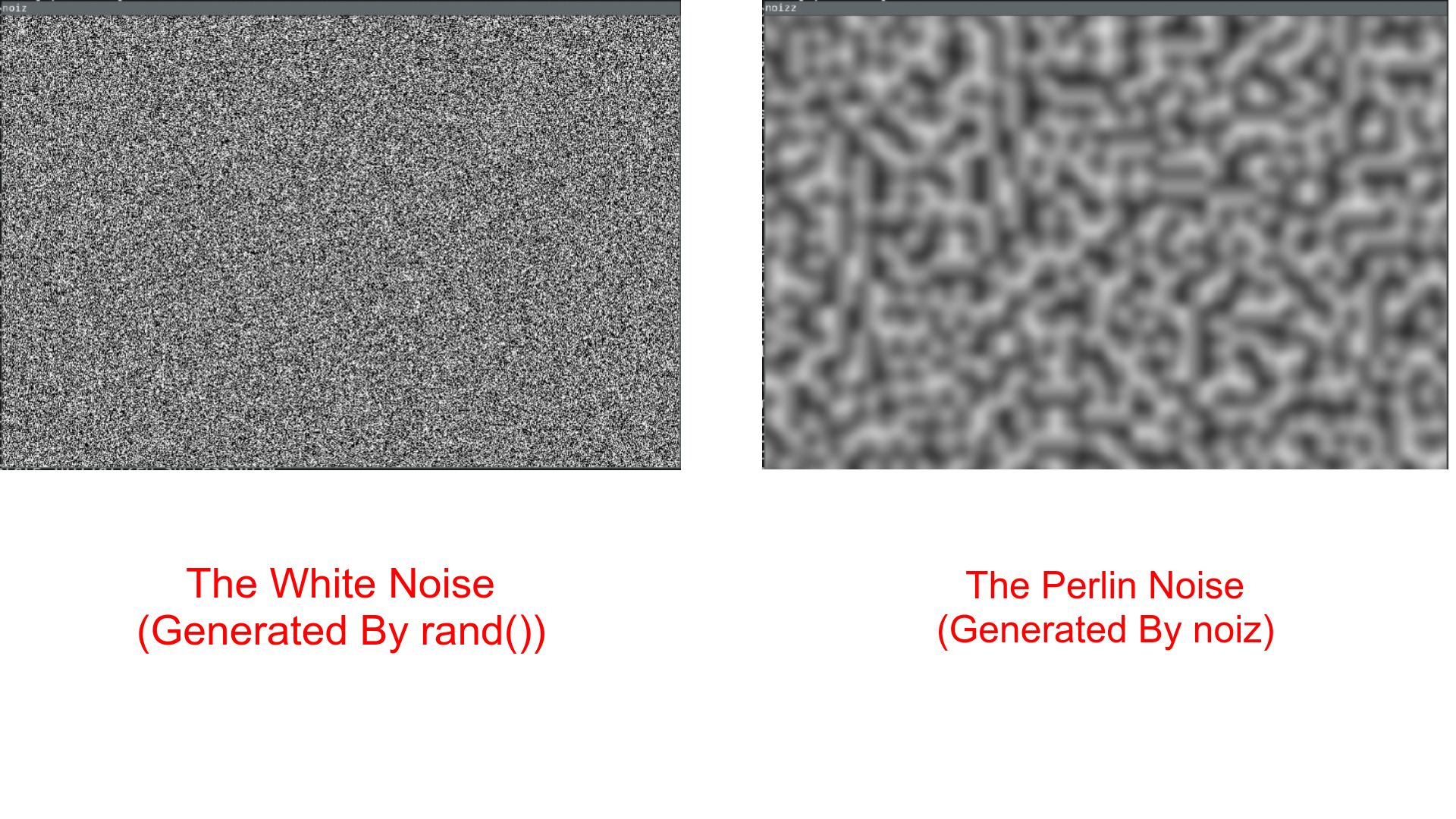
As you can see in the comparative image, Perlin Noise has a much smoother and more natural sound compared to standard white noise.

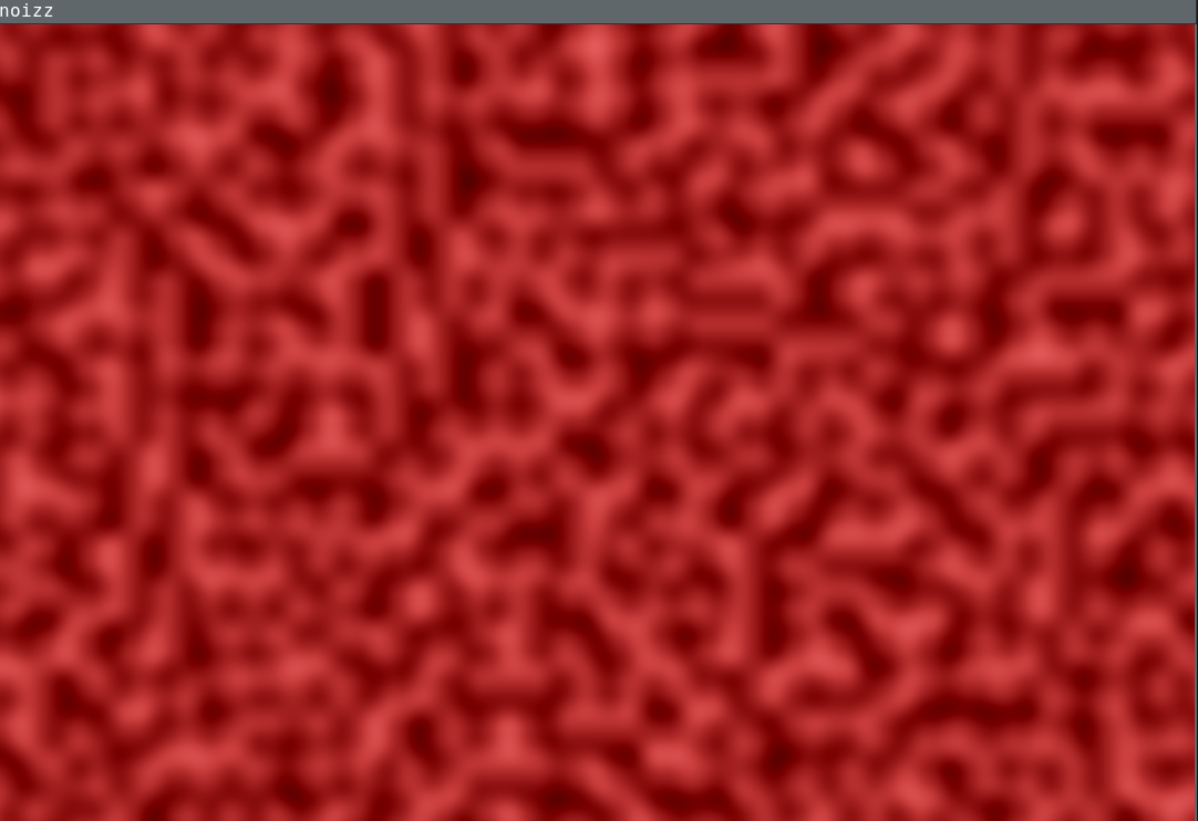
noiz blood

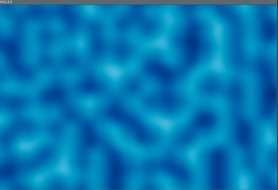noiz ocean

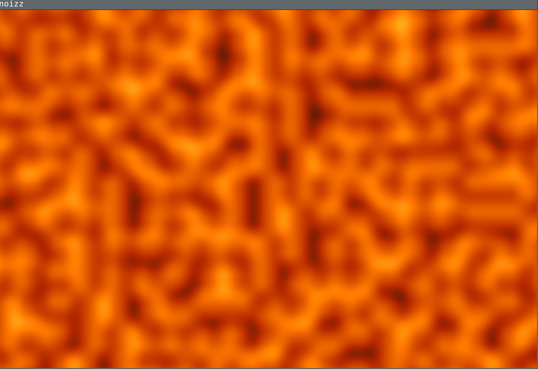noiz lava

Conclusion

I love machines. I love computers. And I love what we can do with them. Perlin Noise is one of the best examples of this. Here, we’re not making the computer less deterministic. With a simple but very cleverly designed algorithm, we trick our eyes and make something very synthetic much less synthetic for us.

I will be sharing the source code of Noizz on my Git server soon. If you want to follow it, you can do so there. Perhaps in the next stage we will expand 2D to 3D and obtain very natural-looking terrains. Until then, farewell.